fmGraphIt
Connect the dots
The Problem
You’ve got a table with a lot of fields, you want to understand how they work together, which fields are used in which calculations, and how the data flows through the table.
How do these fields work together?
I know, that can be quite a time intensive question to answer!
I’m fed up of trawling though field definitions to understand how fields hang together!
How about a diagramme instead? That’d be worth a thousand clicks?
The Solution
fmGraphIt! A way of visualizing data flow and dependencies between the fields of a FileMaker database table.
Just copy the fields and get the big picture with fmGraphIt in just a few clicks!
For example, here are the fields of the communicaton table for telephone numbers, email addresses, etc. in the advanter ERP system.

- A picture is worth a thousand words!
And an interactive diagramme is worth a thouand beers! 🍻
- Click the image to see it in action!
- Hover on a field to see the calculation and other details
What is fmGraphIt?
fmGraphIt is not a single tool, as such - there is no fmGraphIt file - rather, it is:
- a way of displaying field information in a rich, meaningful way
- a process, starting with an XSLT transformation within the fmCheckMate-XSLT library,
- a set of mapping files to implement those display conventions within the yED graphing tool.
Installing fmGraphIt
To generate a field dependency graph from the field definitions of one table you will need
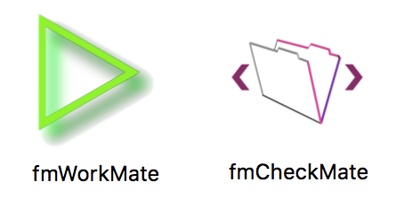
fmGraphIt is part of fmWorkMate and the fmCheckmate-XSLT library. If you already have them, you can skip this step.
-
Install and Setup the fmWorkMate toolbox (which includes the fmCheckMate tool)

-
Install MrWatson’s fmCheckMate-XSLT Library (which includes the graph creation function)

To visualise this field dependency graph you will need a graph visualisation tool.
-
The free yEd software from yWorks
-
Download the latest version of yEd from yWorks
-
some yEd configuration files for formatting the graph (which are to be found in the xml/yEd folder of The fmCheckMate-XSLT Library)
-
Finally, you need
- A step-by-step guide to installing fmGraphIt ( fmWorkMate, the fmCheckMate-XSLT Library, and yEd)
- A tutorial on creating your first Field Dependency Graph
- A Field Dependency Graph Legend
- An introduction to yEd
👌 OK, we are finally ready to go!
Disclaimer and Limitations
Disclaimer:
fmGraphIt’s field dependency graphs are not rocket science—they’re not always perfect—but they provide a quick overview of field structure without needing to create a DDR.
Since the FileMaker clipboard only contains field calculations as a string, the calculation must be parsed. fmGraphIt builds its list of field dependencies by simply (but smartly) searching for occurrences of field names in the calculations.
Limitations:
- False positives: fmGraphIt might falsely interpret text in the calculation (a comment, relationship name,r function name, etc.) as a field reference, if the text matches.
- Relationships are ignored. If a referenced field in a related table has the same name as a field in the current table, fmGraphIt may incorrectly consider this as a reference to the current table’s field.
See How fmGraphIt works for more details on its limitations.
Disclaimer
Before you jump into fmGraphIt you should understand its limits.
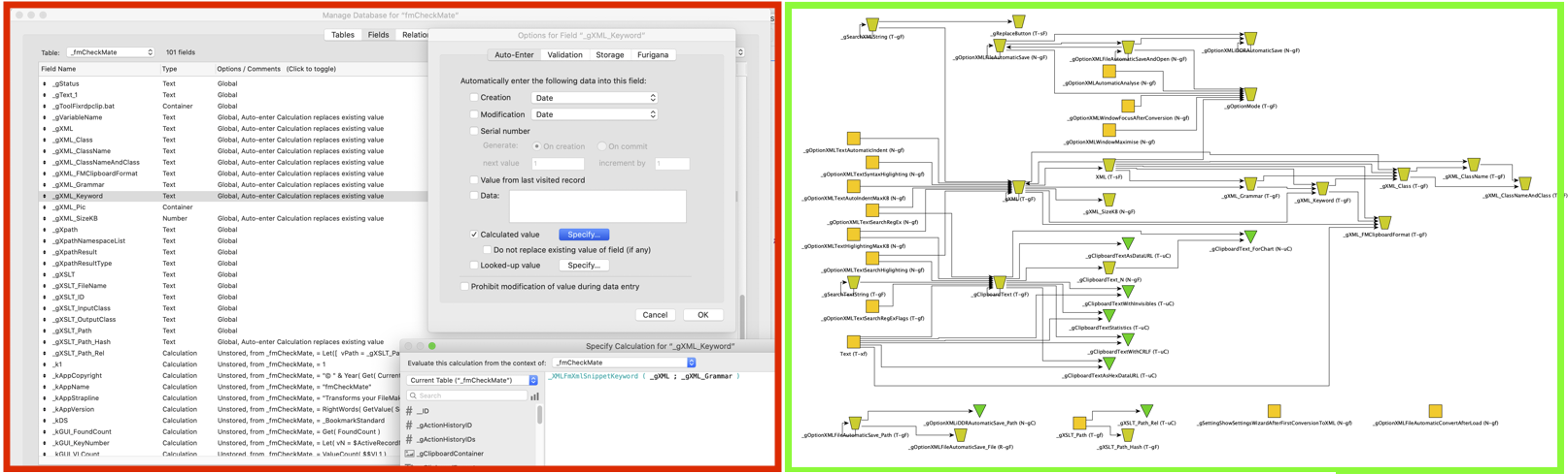
Getting Started
Once you’re set up, you can transform your fields into a stunning diagramme with just a few clicks
- Create a graphml file of your fields with fmCheckMate
- Copy the fields of a table you are interested in
- Convert to XML with fmCheckMate
- Press
[T]and apply the TransformationAnalyse > Fields > Create field dependencies graph advancedto create a graphml Field Dependency Graph- This saves the
Clipboard.graphmlfile to your documents folder, and opens it with the default editor (yEd)
- This saves the
- Visualise the graph in yEd
- The graph is initially displayed in yEd as a pile of dots
- No problem, that’s normal, read on.
- Apply style to the graph
- Open the property mapper with
Edit > Properties Mapper… - Apply the standard style
- Select
FDG: Template = Default (Node) - Click
[Apply]
- Select
- Click
[OK] - You’l see the dots get shape and colour, but are still all in a pile…
- Open the property mapper with
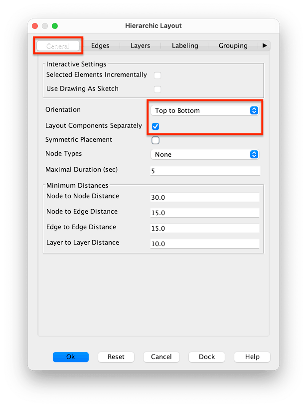
- Now apply a layout-strategy (
Hierarchicalis the best layout for showing data flow)- Select menu item
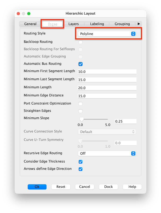
Layout>Hierarchalor press ⌃⌘H - Check the settings, particularly the
GeneralandEdgessettings:
- Select menu item
- Click
[OK]and watch the graph come to life!
- The graph is initially displayed in yEd as a pile of dots
You should see something like the example graph below.
Common issues and tips:
Layout cramped or oriented?
- Try tweaking the layout settings for the best look:
General>Orientation:Top to Bottom- recommended (because of the downward pointing triangles), particularly on smaller graphsLeft to Right- can work better with many fields or long field names
Edges>Routing Style:Polyline- the default, and good for most graphsOctilinear- gives the graph a circuit-board look: great for nerds 🤓
- Alternatively try a different layouting strategry
One-Click Layout- yEd does its best to find the right layout for your dataOrganic- to discover the complex bitsCircular- to see the loops
Too complex?
- Over full graphs can be difficult to navigate, so try to simplify the graph by removing some fields
- Copy less fields to the clipboard in the first place
- Remove all fields that have no dependencies (no arrows in or out)
Want to focus?
-
Zoom in on a particular area of the graph
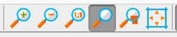
- Select the magnifying glass tool
- Then select the nodes you want to zoom in on
- To return to the full view click the zoom out button on the right
-
Select the field you are interested in and study its connections
- Use the
Context Viewsfrom theWindowsmenu to focus on certain connections Neighbourhood- shows the input / output fields around the selected fieldPredecessors- shows the tree of input fields which feed the selected fieldSuccessors- shows all the output fields of the selected field
- Use the
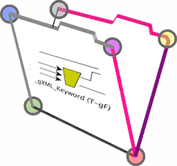
Example Field Dependency Graph
The diagramme shows the field dependencies, or rather the data flow from the (squarish) input fields at the top to the (triangular) calculated output fields at the bottom.
Legend
Here is the legend to the shapes, colours and codes used in the graph:

(Click the image for a large view)
fmGraphIt Field Dependency Graph Explained
Here is how to read the graph…
Field Labels
Each field is labelled with its name and some (cryptic but succinct) metadata:
«field-name»(«data-type»-«storage-type»«field-type»)
Data Type
That’s the same letter as the shortcut key for the data type
The data type is indicated by the following codes:
T- Text
N- Number
D- Date
I- Time
M- Timestamp
R- Container
Storage is also indicated by the colour
Storage Type
Storage is indicated by the following codes
$- $-variable (
$-for script variable and$$for global variable) g- global
s- stored
x- indexed (small x = single index)
X- indeXed (large X = double index)
u- unstored
Field type is also indicated by the shape
Field Type
The type of field is indicated by the following codes
O- an initialised Output field (auto enter & no overwrite & no modification)
o- an initialised once field (auto enter & no overwrite but modifiable)
f- a normal (input) field (small f = no frills)
F- a Filter Field (large F = with auto enter & overwrite)
C- a calculation field
S- a summary field
For variables the following codes are used (or rather will be one day):
-- a $-script variable
$- a $$ global variable
Shapes
The pointier the shape, the more complex the type of field.
⏺️→⏹️→⏢→▶️→*️⃣
The shape indicates the field type:
- ⏹️ Square shapes are input fields
- ▶️ Triangular shapes are output fields
- 🔼 Upwards pointing are data source fields (locked + initialised fields, creation date, etc.)
- 🔽 Downwards pointing are data aggregators (calculation fields)
- ⏢ ‘Tweeny’ shapes are a bit of both
- 1/2 ⏹️ + 1/2 ▶️ = 1/2 input + 1/2 output = Auto-Enter fields
- *️⃣ Star shapes are summary fields
- ⏺️ Circle shapes are variables.
See the Field Depency Graph Legend for more details.
More colour → more storage
lighter → less CPU
darker → more CPU
Colours
The colour indicates the storage type, and follow these simple guidelines:
See the Storage vs CPU part of the legend for more details.
Top to Bottom Layout Orientation
Data flows from top to bottom
The shapes of the fields have been chosen to fit a top-down hierarchy well visually.
- At the top you find
sourceandinputfields`:- 🔼 non-modifiable metadata fields (‘output’ source fields)
- ⏹️ normal input fields (with/without Auto Enter)
- In the middle you find fields that build on the source + input fields:
- ⏢ auto-enter fields
- 🔽 calculation fields
- Towards the bottom you find the deeper ‘aggregator’ fields:`
- 🔽 calculation fields
- *️⃣ summary fields
Note: The arrows show data flow rather than dependency
Tooltip - Calculation Type
In the calculation in the tooltip, the kind of ‘equals sign’ used indicates what kind of calculation it is:
=- Calculated field
:=- Autoenter field
<=- Lookup field
Note: This is a subset of the fmCheckMate Print fields function
_ID :+1 7- A field with auto-incremented serial number (Auto-Increment)
active : "1"- A field with an auto-enter fixed text (Auto-Data)
Status := "New"- A field with an auto-enter initial calculated value (Auto-Init)
DateDeparture :== DateArrival+2- A field with an auto-enter filter calculated value (Auto-Calc)
Info :=== "Input: " & Quote(Input)- A field with an auto-enter filter calculated value even when inputs empty
RepIndex = ArrIndex+1- A calculated field
_sTotal =∑: Score- A statistic field = Total
_sCount =N: Options- A statistic field = Count
_sAve =∑/N: Score- A statistic field = Average
_sMin =≤: Score- A statistic field = Minimum
_sMax =≥: Score- A statistic field = Maximum
_StdDev =σ: Score- A statistic field = Standard Deviation
_Frac =½: Score- A statistic field = Fraction of Total
_List =∑¶: Names- A statistic field = List of Text
Enjoy!
MrWatson